
The Role of Machine Learning in Classifying Animal Movement
Modern ecological research relies heavily on advanced computational techniques to interpret vast streams of telemetry data. Understanding the role of machine learning in classifying animal behavioral patterns allows scientists to transform raw sensor readings into meaningful insights. This page explores how automated algorithms process complex movement traces to identify specific activities, overcome field data challenges, and advance our knowledge of wildlife ecology.
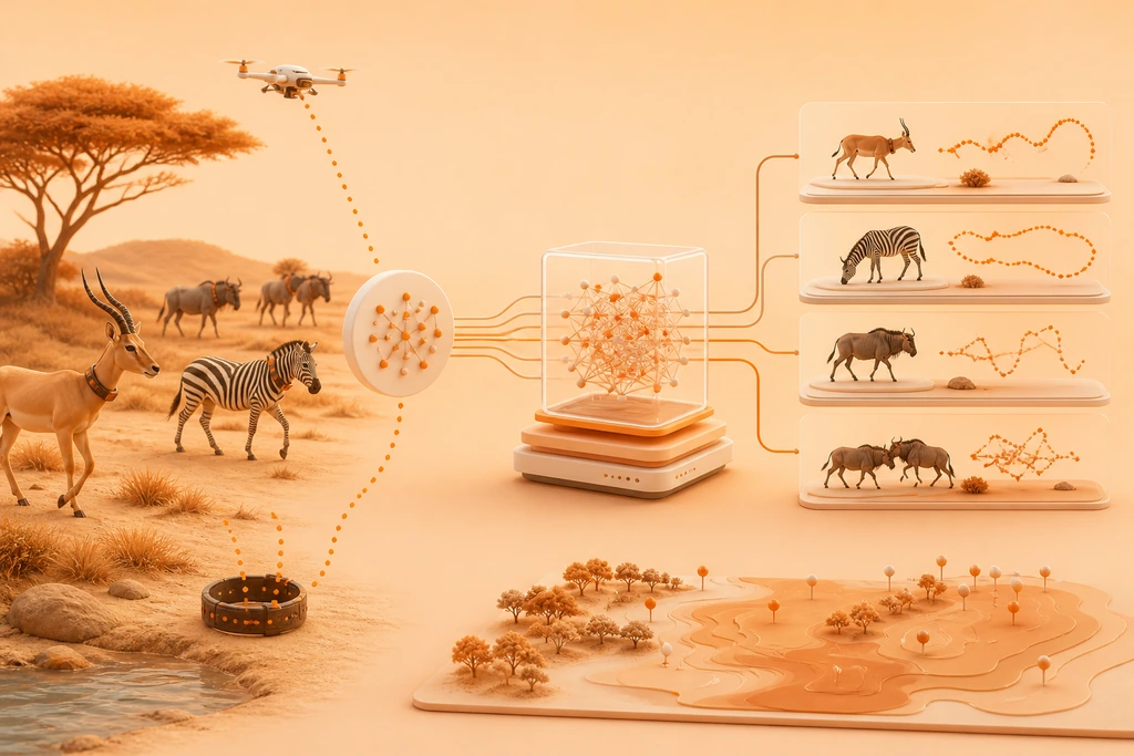
Machine Learning in Animal Movement
-
Clean raw sensor data
Engineers clean raw voltage and positional coordinates from collars. They remove dead sensor pixels, temperature offsets, and low-battery voltage drops before analysis.
-
Extract movement features
The model extracts key features from high-frequency accelerometer streams. It calculates orientation, dynamic body acceleration, and turning angles to represent motion.
-
Train classifiers with labels
Field observations and video footage provide ground truth labels. Supervised algorithms learn to map specific sensor patterns to actual animal behaviors.
-
Evaluate model classification performance
Researchers test the trained classifiers against independent datasets. They measure accuracy in detecting foraging, resting, and migrating states in harsh conditions.
-
Deploy models in field conditions
Optimized algorithms run on edge devices or post-processing pipelines. The system classifies continuous behavioral patterns of free-ranging wildlife remotely.
Signals hidden in movement traces
A collar or a tag does not record behaviour directly; it records voltage and positional coordinates. A tri-axial accelerometer sampling at frequencies between 10 and 50 Hz generates millions of raw data points per animal every single day, while a GPS receiver adds a parallel stream with its own clock drift and satellite geometry constraints. Before any predictive model can process this stream, engineers must clean the raw trace thoroughly. Dead sensor pixels, temperature-induced offsets, and extended periods of low battery voltage all masquerade as unusual biological motion. Furthermore, physical device placement critically influences the output data because a tag mounted on the neck swings quite differently from one attached to a dorsal fin or a wing. Classifiers trained on one specific mounting position rarely transfer successfully without recalibration. Analysts typically segment the cleaned trace into short temporal windows lasting two to ten seconds, calculating summary statistics such as mean, variance, jerk, and dominant frequency for each segment.
How labels teach a classifier
Supervised learning algorithms require dependable training examples to map input metrics to real-world actions. In field research, this means dedicated observers watching video recordings or focal animals directly, marking second by second when an individual walks, grazes, flies, or rests. The resulting dataset pairs each distinct time window with a specific behavioural label, allowing the model to establish classification boundaries. Random forests and gradient boosting remain popular workhorses for tabular feature sets, whereas one-dimensional convolutional networks and spectrogram-based CNNs process raw waveforms directly. Hidden Markov models are frequently integrated because they encode temporal continuity, acknowledging that a grazing bout rarely lasts merely a fraction of a second. Two critical operational warnings must be noted: human-assigned labels contain noise, with independent observers achieving inter-observer agreement only 80 to 90 percent of the time, and target behaviour classes are heavily imbalanced, since resting periods frequently dominate the recording logs. Before training a model, researchers often rely on specialized methodologies-for-processing-complex-spatiotemporal-animal to handle large volumes of spatial telemetry data.
Thresholds versus trained classifiers
Two distinct analytical approaches compete for the same ecological monitoring task, and choosing between them requires careful evaluation of project constraints. Consider a simple rule that flags flight whenever overall dynamic body acceleration exceeds a specific numerical limit for more than five seconds. Such a threshold is completely transparent, demands no training dataset, runs efficiently on constrained microcontrollers, and can be explained easily to reviewers. Conversely, a machine learning classifier trained on thousands of labelled windows successfully captures complex postures, intermittent movement variations, and sensor tilt angles that rigid thresholds miss entirely, typically lifting balanced accuracy significantly on identical recordings. A pragmatic middle ground involves using initial thresholds to inspect raw data and catch gross sensor faults, then transitioning to a learned model once sufficient labels are gathered. Always retain the simple threshold as a baseline comparison metric; if the advanced classifier fails to outperform this basic baseline on held-out test subjects, the added computational complexity is unjustified.
Machine Learning for Animal Movement Analysis
| Data Input Type | Processing Step | Model Application | Operational Challenge |
|---|---|---|---|
| Tri-axial accelerometer and GPS streams | Cleaning raw sensor traces | Classifying movement patterns | Managing clock drift and low battery |
| Raw voltage and positional coordinates | Extracting key behavioural features | Training supervised classifiers | Handling temperature-induced sensor offsets |
| Millions of daily data points | Filtering dead sensor pixels | Distinguishing behavioural states | Processing high-frequency sampling rates |
| Unprocessed positional telemetry | Calibrating spatial coordinates | Running unsupervised clustering | Overcoming satellite geometry constraints |
Four features worth extracting
Feature engineering remains the primary determinant of model performance, particularly when working with relatively modest training set sizes. Four distinct feature categories capture the vast majority of useful ecological signal.
- Dynamic acceleration — overall dynamic body acceleration and vectorial DBA, computed after a low-pass filter separates gravity from movement, summarised per window.
- Attitude — pitch and roll derived from the static component, which distinguishes standing from lying, or soaring from flapping.
- Rhythm — dominant frequency and its amplitude, catching wingbeat rates that fall between 3 and 12 Hz for many birds.
- Path geometry — GPS speed, turning angle and tortuosity, which separate commuting flights from area-restricted searching.
This structural phase represents the practical core of the role of machine learning in classifying animal movement patterns: predictive models do not invent biomechanical principles on their own; rather, they intelligently weigh the specific descriptors supplied by the researcher.
Classifying behaviour without labels
Not every ecological research initiative secures the funding required to generate thousands of hours of manual behavioural labels, meaning some of the most innovative analytical results originate from unsupervised learning methods. Algorithms like K-means clustering or Gaussian mixture models applied over window features frequently recover distinct recurring modes — such as resting, slow travel, fast travel, and localized searching — that researchers map to biological behaviours retrospectively. Hidden Markov models extend this unsupervised capability further by explicitly modelling state transitions, producing an output sequence of behavioural states complete with realistic dwell times rather than isolated independent guesses for every temporal window. Modern self-supervised approaches, where deep networks learn to predict subsequent temporal windows or match augmented views of identical movement bouts, now generate robust embedding spaces that a simple linear classifier can separate using only a minimal fraction of labelled examples.
Machine Learning in Animal Movement
Processing raw sensor data streams
Training classifiers with expert labels
Overcoming rigid threshold limitations
Extracting key behavioural features
Applying models in field conditions
Machine learning in field conditions
Deployment phase is where promising analytical models frequently fail under harsh environmental conditions. Wildlife tracking tags operate under strict energy budgets, meaning raw high-frequency sensor data rarely leaves the physical device; instead, inference executes directly on the onboard microcontroller, and only summarized metrics or detected behavioural events are transmitted over satellite links. Quantising a neural network from floating-point precision to integer formats successfully reduces memory consumption and battery draw, usually incurring only a minor drop in accuracy that must be measured empirically rather than assumed. A quieter yet more dangerous failure mode relates to poor spatial or temporal generalisation. Randomly splitting windows from the same recording artificially inflates validation scores because adjacent windows share near-identical sensor signatures. True field performance depends strictly on splitting training and test sets by individual animal, seasonal timeframe, or geographical deployment site. Publishing exact feature lists, window lengths, and firmware versions alongside performance metrics ensures scientific reproducibility.